Changepoint Detection
Some things never change.
Happy New Year (although by the time this post goes live it’ll be halfway through January, so it’s probably becoming a bit too late to be wishing a HNY).
It’s January. A month where many pledge to make positive changes in their lives (more gym sessions, less alcohol etc). Given this I thought a fitting first blog post of the new year would be about change, more precisely changepoint detection (that was a tediously linked introduction, buy hey some things never change).
I finished my PhD on Changepoint Detection in 2017, it is now 2020 and you would think I would have stopped raving about them by now, but actually I think I like and appreciate them more now than I ever did back then. They’ve become a common data transformation step in my data science workflows that I thought I’d write this blog post as an introduction to changepoint detection as well as show how I use them day to day.
I think my appreciation of changepoint detection has grown in recent years whilst I’ve been faced with real life, sometimes large, and messy data sets. During my PhD I was sheltered by nice clean academic data which contained small amounts of observations with obvious changes I can see the change without using a computer (“hilarious” comment from an audience member during every changepoint detection presentation ever given). Most changepoint detection projects all used the same oil or financial data set and it was difficult to see what the point really was.
It wasn’t until I started trying to forecast demand for 1000s of product and location combinations that I really started to understand the need for changepoint detection. Demand of products naturally change over time due to what is hot and what is not. Detecting these changes in demand allows us to use data which best resembles the current state of play meaning we don’t wrongly skew the forecasts by historic demand patterns.
What are changepoints?
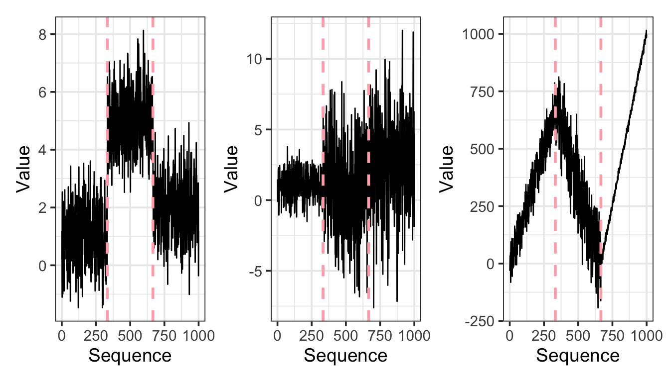
Changepoints are points in sequences of observations where there has been some sort of change on the distribution of the data points. For example changes in mean, variance and/or trend, as shown in the plots below.
Detecting changepoints in practice
Changepoint detection in practice is useful during the transformation steps, so when you are cleaning your data pre modelling. It can also be useful on post event analysis for testing whether some intervention or business change had an impact. For example if you are a retailer you might want to see whether introducing a promotion changed the number of sales.
Cleaning data before modelling and post event analysis are two examples of offline changepoint detection, this is where the data is collected and then changepoint detection is applied. Changepoint detection can also be run in real time (online) which is useful for data checks to flag when data looks suspicious - maybe the data processing step has stopped running or has produced duplicates.
There are many libraries available for running changepoint detection in R, this recent blog post gives a high level overview to some of these https://lindeloev.github.io/mcp/articles/packages.html.
In python this blog highlights a few options https://techrando.com/2019/08/14/a-brief-introduction-to-change-point-detection-using-python/ the best looks like the ruptures package which is an adaption of the changepoint package in R.
There is also a Julia adaption of the changepoint R package https://github.com/STOR-i/Changepoints.jl.
Changepoint Detection in R
My go to package for changepoint detection is the R changepoint package written and maintained mainly by Rebecca Killick with help from various peers at Lancaster University. It is a great all round package for detecting changes in mean, variance and, mean and variance.
This package implements a few methods, I won’t go into details on the inner workings of the methods but check out this paper written to supplement the package https://www.jstatsoft.org/article/view/v058i03/v58i03.pdf.
The changepoint package has 3 classes of models that are all called in similar ways cpt.mean, cpt.meanvar and cpt.var depending if you are expecting, or trying to detect, changes in mean, mean and variance, and variance, respectively.
A brief description of the function arguments and how I tend to use them:
data: the data object that you wish to find a changepoint in. This can either be a vector, time series object or a matrix (if a matrix it is assumed that each row is a separate data set.)penalty: the default penalty value has been chosen to be the “MBIC” (modified Bayes Information Criteria). Usually I leave it as is. Sometimes I will use “CROPS” which is a method I developed with during my PhD which helps to select the best penalty term based on a range of penalties.pen.value: depending on the choice of penalty there might be a requirement to set a penalty value. For example if using CROPS then the pen.value is the range of penalties to search over.method: the choices of methods are AMOC (at most one changepoint), PELT, segment neighborhood search or Binary segmentation. I normally use either AMOC, if I want to only detect one changepoint, or PELT: a method that finds the the optimal changepoint locations and doesn’t take too long to run.Q: an argument required when using binary segmentation or segment neighborhood search, I tend to ignore.test.stat: this can only be set to “Normal” or “CUSUM”. I leave it as the default “Normal”. If the data appears to not follow a normal distribution then instead I’ll usecpt.npfrom thechangepoint.nppackage which is a non parametric approach I developed during my PhD which can be applied to any data set without any underlying assumptions of the distribution of the data.class: If TRUE then an object of classcptis returned. I leave this as it.param.estimates: If TRUE and class is TRUE then the parameter estimates are returned. I leave this as it.minseglen: This is a positive integer which gives the minimum segment length that we will allow. This is useful to control the sensitivity of the changepoint method to recent changes. For example in one of my projects I have set it so that a change with an increase in demand is detected after 1 month at this new level to make sure stock levels are increased to satisfy this demand whereas for a decrease in demand we don’t want to remove stock too soon in case demand picks up so in this case we wait 3 months.
Examples
Below is an example code snippet of how I use changepoint detection in a workflow to pre-process some data and then return the mean of the data.
# initialise some data with changepoints at locations 50, 100, 150 and 200.  (Note this is the suggested example from the `changepoint` package).

set.seed(1)
data = data.frame(seq = 1:200, values = c(rnorm(50,0,1),rnorm(50,5,1),rnorm(50,10,1),rnorm(50,3,1)))

# plot the data to have a look

data %>% ggplot() +
  geom_point(aes(x = seq, y = values)) +
  theme_bw()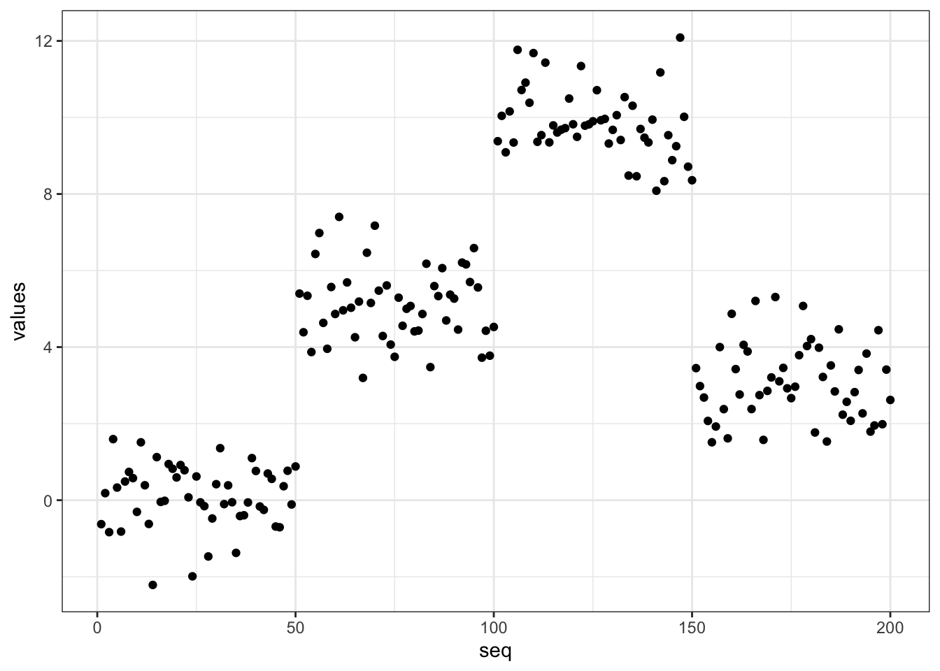
# suppose we are interested in the mean of all values

data %>%
  dplyr::summarise(mean(values))
## mean(values)
## 1 4.53554# Normally in practise I am using changepoint detection so that I am only using the most recent data that will resemble the current state of play- therefore a use a function to remove points previous to this point.
changepoint_transform <- function(data, input_method, input_minseglen){
changepoint_locs <- changepoint::cpt.mean(data$values, method = input_method, minseglen = input_minseglen)@cpts # detects points at 50, 100, 150 and 200
data_post_change <- data %>%
dplyr::filter(seq >= tail(changepoint_locs, 2)[1]) # note the changepoint function returns the last point in the series as a change
return(data_post_change)
}
# now we detect the most recent changepoint and then find the mean. Note this is more representative of the most recent data.
data %>% changepoint_transform(input_method = "PELT", input_minseglen = 10) %>%
summarise(mean(values))## mean(values)
## 1 3.180448I’ve recently started using functions joined together in pipes (%>%) more and more in R as I find it useful for mixing and matching the different steps. For example my workflow might include other functions for doing things like dealing with missing values and/or detecting anomalies.
Changepoint Detection in python
As part of writing this blog I decided I would see if I could in some way replicate what I do in R in python. For this I looked into the ruptures package. In this package you call the changepoint detection method you want to use directly. In this case I use .Pelt. There appears to be 2 steps .fit which segments the signal and then .predict which then returns the optimal changepoint locations. These 2 steps can be done at the same time using .predict_fit.
One thing to note is there aren’t any inbuilt functions for the penalty and therefore a value needs to be passed (or another function used to calculate this). Note for this example I’ve just set it to be 10.
import ruptures as rpt
import numpy as np
import pandas as pd
import matplotlib
import matplotlib.pyplot as plt

# initialise some data with changepoints at locations 50, 100, 150 and 200.  (Note this is the suggested example from the `changepoint` package).
np.random.seed(1)
data = pd.DataFrame(np.concatenate((np.random.normal(0, 1, 50), np.random.normal(5, 1, 50), np.random.normal(10, 1, 50), np.random.normal(3, 1, 50)), axis = None), columns=['values'])

# plot the data to have a look
fig, ax = plt.subplots()
ax.plot(data)
plt.show()

# suppose we are interested in the mean of all values 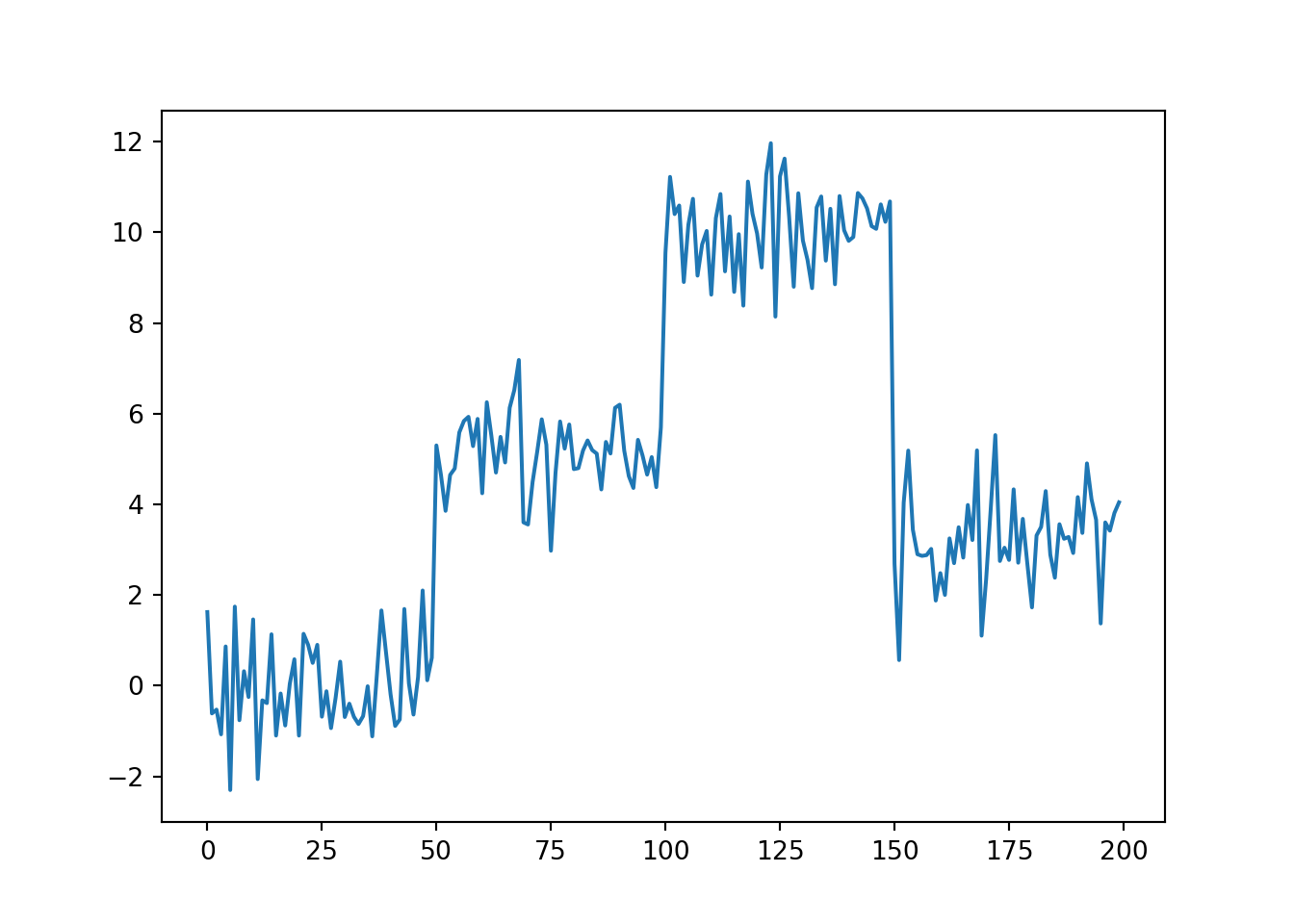
data.mean()

# Normally in practise I am using changepoint detection so that I am only using the most recent data that will resemble the current state of play- therefore a use a function to remove points previous to this point.
## values 4.606689
## dtype: float64def changepoint_transform(data, input_min_size):
changepoint_fit = rpt.Pelt(min_size = 10).fit(signal = data)
changepoints_locs = changepoint_fit.predict(pen = 10)
return data[changepoints_locs[-2]:]
# now we detect the most recent changepoint and then find the mean. Note this is more representative of the most recent data.
changepoint_transform(data, input_min_size = 10).mean()## values 3.220931
## dtype: float64This code replicates what I would do in R but in python. I’m still learning best practice in python so maybe I would use this package or maybe I would just call the R functions, given I have a lot of confidence in how these work, using the rpy2 package. I’m also still getting my head around methods and functions in python so I haven’t worked out if I can chain the functions together like I have done in R.
(It excites me that thanks to the reticulate package in R it is possible to run python code within this R markdown script which is very cool!)
Conclusion
There is so much more I could cover in changepoint detection but hopefully what I have detailed in this post will have convinced you that changepoint detection is a useful tool especially in pre-processing of data. I have given a couple of examples of how to use in both R and python which should provide a good place to start.
Kaylea Haynes
Data Scientist
I know quite a lot about time-series analysis, demand forecasting and changepoint detection but I’m currently trying to broaden my data science skills.